Grouping Data in a Pivot Table

The Pivot Table in Google Sheets after the latest updates is now a powerful tool for grouping and summarising a large set of data. The first three are configured by you in the backend of the report.

How To Create A Pivot Table For Data Analysis In Microsoft Excel Data Analysis Pivot Table Data Analysis Tools

Setting up the Data.

. This enables us to analyze summarize calculate and visualize trends comparisons and patterns in our data. Do NOT check the box to add the data to the Data Model. In our example we are going to use the price as the row label and the number count of transactions in the value area.

Next create a pivot table with the field you want to group on as a row label. This is not helpful. In the pivot table shown there are three fields Name Date and Sales.

Pivot Table Group by Month. If you are using Excel 2016 its probable that the data is going to be displayed in a different format than its formatted inside a table. You can generally ungroup grouped Pivot Table data in the following 3 easy steps.

In the example shown the pivot table is uses the Date field to automatically group sales data by month. On that screen enable Add to data model option. If your data is in different workbooks or worksheets you have two ways to get a pivot table from it.

Click ok to insert pivot table. Lets say you want to group all the dates as months instead of adding a different column in your data its better to group dates. Note that the values column has COUNT instead of SUM.

For example change the date grouping in the first pivot table to Months and the dates in the second pivot table automatically group in Months. Once the date field is grouped into years and quarters the grouping fields can be dragged into separate areas as seen in the example. Sorting date range table filters and dashboard controls.

Right-click on an Item within the group you want to ungroup. The steps below will walk through the process of Grouping Pivot Table Data by Month. Figure 1- How to Group Pivot Table Data by Month.

The process for creating this Pivot Table is as follows. The first one gets all the data in a single sheet by copy-paste and then make a pivot table from it. Apart from months you can use years quarters time and even a custom date.

I will walk through how you can progress from a simple aggregate query to a PIVOT query that returns this identical output colors and styling aside which are still the. By grouping dates in a pivot table you can create instant reports. Hello I was trying to follow the steps listed in the Copy a Pivot Table and Pivot Chart and Link to New Data article but after re-linking the copied pivotchart excel 2007 simply remove the old pivotchart formating colors labels captions etc.

We will create a Pivot Table with the Data in figure 2. Excel displays a contextual menu. If you want to ungroup a manually-grouped Field right-click on the Field header.

Once grouped together you can drag the group to your Pivot Table and start your analysis. With data in place lets say you want to produce a report that looks like this with totals within data centers and overall rolled upward and no data center names repeated. Select any cell within the data range or select the entire data range to be used in your Pivot Table.

The time grouping feature is new in Excel 2016. To build a pivot table to summarize data by month you can use the date grouping feature. Create the Pivot Table.

When properly configured with filters the numbers in a pivot table show the big picture and help clients answer specific business questions. There are a few ways to organize and filter data in your pivot table. Then when you refresh the pivot table it will include all of the data in the range even if new rows have been added.

In the example shown a pivot table is used to summarize sales by year and quarter. When you go through the process of grouping this time you will see that it allows the 2 grouping types to exist on the same source data. If you are unfamiliar with grouping dates into months weeks etc directly within a pivot table have a look at the Pivot Table Course.

The Pivot Table enables the users to generate awesome reports in Google Sheets without using any formula their own. Add the field you want to distinct count to the value field area of the pivot table. Keep the OLAP-based pivot table too and youll have two pivot tables based on the same data using different pivot caches.

This will give you a Pivot Table as shown below tabular form. In any sector data is captured on a daily basis so when we need to analyze the data we use pivot tables so it will also summarize all the dates and give every single day but who will sit and see everyday transactions rather they want to see what is the overall monthly total which comprises of all the dates in the month and gives the single total for each. The following example creates a pivot table that displays the total sales for each month of the year broken down by sales region and sales rep.

As you can see from the picture below our resulting pivot table has individual prices. How To Ungroup Grouped Pivot Table Data. If you want to change it right-click and then ungroup Ungroup PivotTable Tools Analyze Group Ungroup.

With time grouping relationships across time-related fields are automatically detected and grouped together when you add rows of time fields to your PivotTables. Using this data Ive created a Pivot Table with Stores and Sales in the Rows area and Sales in the Value area. Figure 2 Setting up.

Create a second pivot table from the source data. If you want grouping youll need a pivot table with its source data NOT added to the data model. Now heres the good news.

Solution 2 grouping cells in PivotTable. Select your data and go to insert pivot table screen. Because you created the two pivot tables from the same source data by default they use the same pivot cache which is where the grouping is stored.

Another one is to use this feature of MS Excel wizard. Pivot tables have a built-in feature to group dates by year month and quarter. Go to value field settings and select summarize by Distinct count Here is a video explaining the process.

Option 1 -- Named Table In Excel 2007 and later versions you can format your list as a Named Table and use that as the dynamic source for your Pivot Table.

Learn How To Quickly Extract Valuable Insights By Slicing Filtering And Grouping Your Data Using Pandas Pivot Tables Pivot Table Data Data Science

Half Way Through Manual Grouping Group 1 Is Done Pivot Table Excel Microsoft Excel

Use An Excel Pivot Table To Group Data By Age Bracket Pivot Table Excel Helpful Hints

Pin On Excel

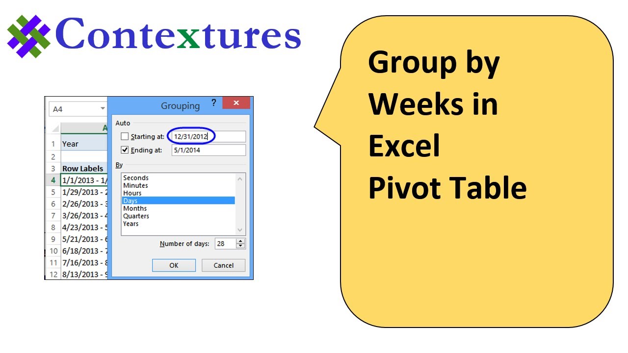
Group By Week In Pivot Tables Pivot Table Online Lessons Excel

How To Group Pivot Data By Month Pt 1 Pivot Table Data Labels

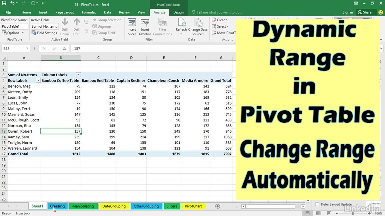
Automatically Change Range Of Pivot Table When Data Is Added Microsoft Excel Tutorial Youtube Excel Tutorials Microsoft Excel Tutorial Microsoft Excel